DISCLAIMER:- This post is an excerpt from my capstone project report from my bachelors degree. Harish Kumar, Gokull Subramanian, and I were the contributors.
If you are interested in reading the full project report, it can be found here.
Libraries used:- Python, OpenCV, TensorFlow, PyTorch, Keras
Motivation
Autonomous vehicles as well as vehicles with ADAS features use multiple sensors and integrate their data to take decisions and assist in the driving process as well as in automating it. By using LiDAR, RADAR, etc., data can be acquired in metric units which helps in taking decisions in real world environment. However, the high cost of such sensors is a major drawback. In the recent years, researchers as well as autonomous vehicle manufacturers have been looking at the feasibility of using only RGB cameras for perception. This is largely attributed to the influence of deep learning on computer vision in the current decade. This project work has been focused on the perception aspect of autonomous vehicles with data from a single RGB camera.
Objective and Challenges
Our primary objective was to predict the semantic activity of the ego vehicle as well as the vehicles on the scene. The goal was to build an end-to-end activity classifier using a video object segmentation approach which could do object detection, semantic segmentation as well as instance level tracking and then we planned to use those information to predict the activity. But the first challenge was to find a common dataset which contains ground truth labels of object lables, pixel level labels as well as pixel level optical flow labels. At that time such dataset did not exist.
So our objective was achieved using three deep neural networks for three tasks namely, object detection and tracking, lane detection and optical flow estimation. Object detection and tracking was used to detect and track the vehicles on the scene. Lane detection was used to understand the context of the road. Optical flow estimation was used to capture the motion of vehicles. The outputs of the three networks were manually integrated to interpret the semantic vehicle activity. The secondary objective was to run this integration on an embedded board. The performance of the same was evaluated and the results were presented.
Proposed Pipeline
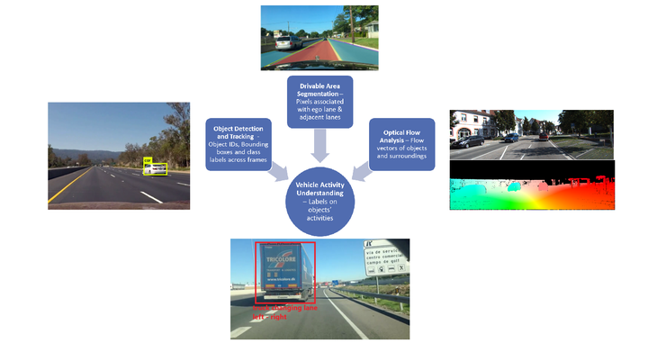
Understanding of semantic vehicle activity required information about the objects in the scene, their motion and the information about the road itself. This information should also be temporal (related across frames) which is why tracking plays an important role too. The object detection network gives the classes of the detected objects and provides bounding boxes to the tracking algorithm as input. The tracking algorithm uses these bounding box coordinates to track these objects across frames. The lane detection algorithm detects all the visible lane markings on the scene in a distinct manner such that the ego lane can be detected in every frame. Optical flow estimation provides the flow vectors of each pixel in the frame as input to manual integration. An abstract model of the proposed pipeline is given in below figure.
 |
|---|
| Figure 3.1: Proposed Pipeline |
 |
|---|
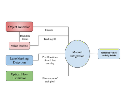
| Figure 3.2: Integration Pipeline |
Object Detection and Tracking
Problem Definition
Semantic understanding of vehicle activity demands identification of the vehicles in videos. Object detection can be used to detect objects in each frame and tracking can be done to associate the data acquired from object detection along all the frames.
A tracking by detection approach was proposed to do object detection and tracking as two different tasks. Object detection involves classification and localization of objects in an image. Tracking algorithm tracks multiple objects across all the frames.
Need for the Task
Object detection is an important task in scene perception and it is done across all frames for the following reasons:
- To classify the objects present in the set of pixel areas.
- To localize the objects using a bounding box in an image.
Tracking is essential for the following reasons:
- In order to associate the information acquired from object detection from all frames and get a tracking ID for each object.
- To track the objects along successive frames until they exit the field of view of camera.
- To mitigate the effect of identity switches caused by occlusion, motion blur, lighting conditions.
YOLO Network Architecture
YOLO is a single shot object detector, which takes image as an input and gives a tensor containing all bounding box information, classes and confidence scores.
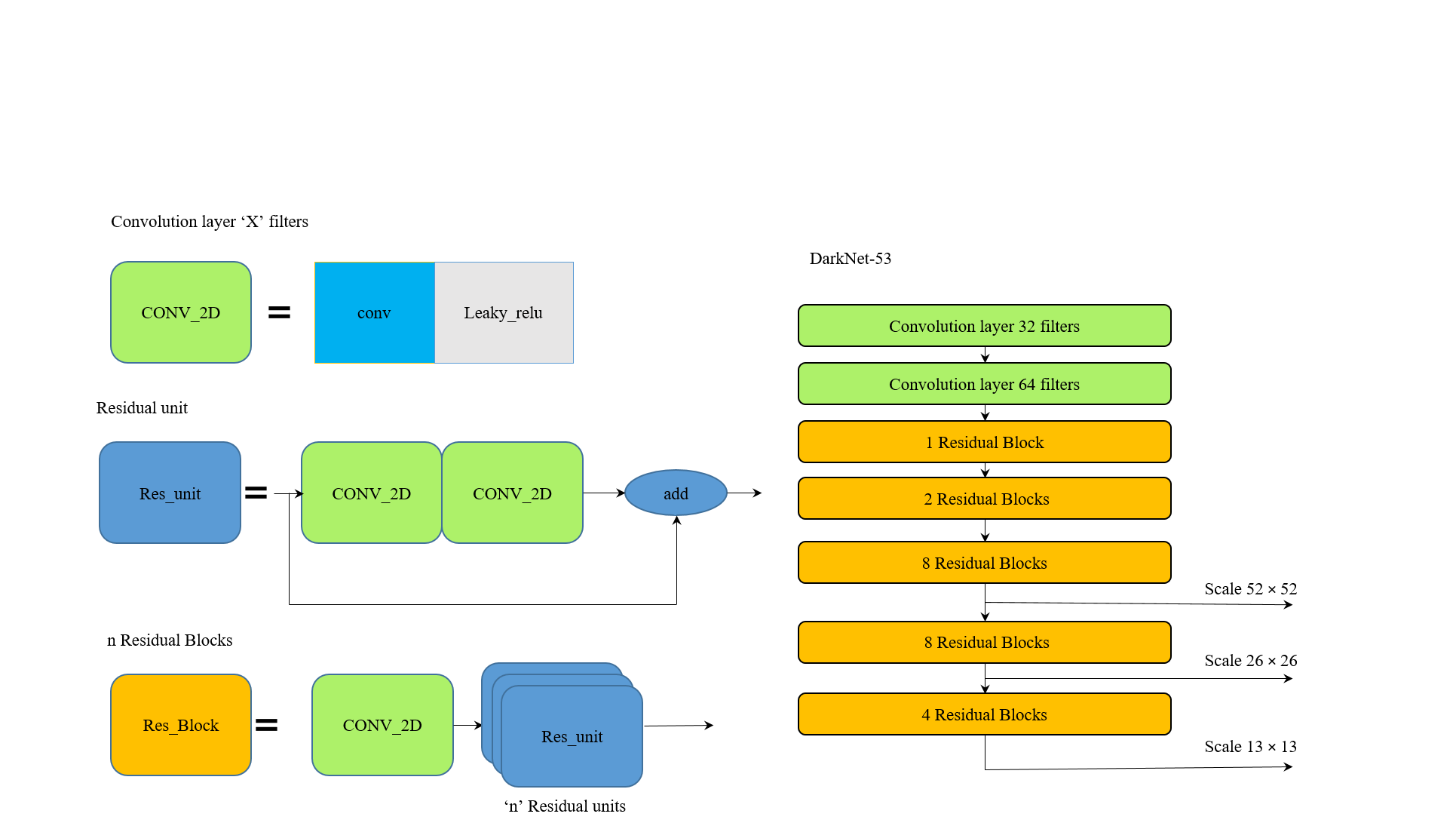
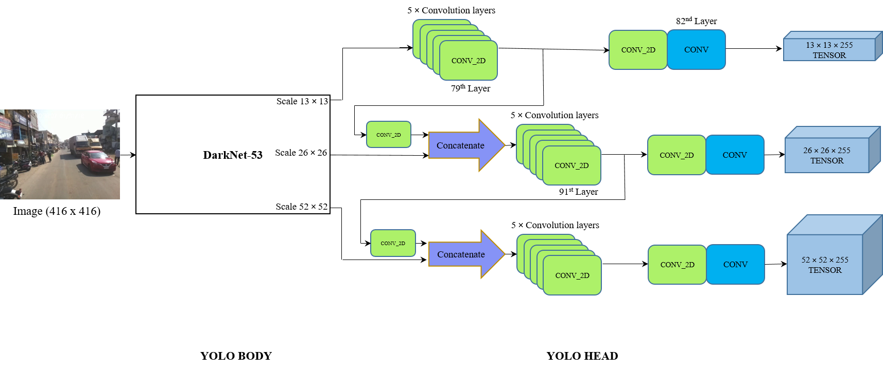
To understand YOLO network architecture, it can be divided into two parts such as YOLO body and YOLO head. First part of the architecture is used to extract features, which is considered base network. In YOLOv3, Darknet-53 has been used as base network, also called as YOLO body, to extract features from the input data. Then the extracted features will be subjected to YOLO head, which does the detection of objects. This detection involves the localization and classification of objects.
YOLO body (DarkNet-53) extracts features from an image in three different scales for detecting small, medium and large objects accurately, which will be fed into YOLO head.
To simplify DarkNet-53 architecture, it has been divided into CONV2D blocks and Residual blocks as shown in Figure.
 |
|---|
| Figure 3.2: DarkNet-53 Architecture |
Each CONV2D block consists of a convolution layer along with a leaky ReLU layer as in Figure. Residual blocks (Res-Block as per the Figure) are made of one 24CONV2D block followed by n residual units. Here, n defines the number of residual blocks. Each Residual unit can be made by two CONV2D blocks stacked together and added with the input itself.
 |
|---|
| Figure 3.3: YOLO v3 Architecture |
YOLOv3 generates 3 different scales of output tensors containing the bounding boxes, confidence scores and class names. This output tensor will be subjected to few post-processing steps such as IoU and Non Max Suppression (NMS) to remove the unnecessary bounding boxes. Bounding boxes, class names and confidence scores will be found from object detection. Bounding boxes from object detection will be used for tracking.
Deep SORT Algorithm
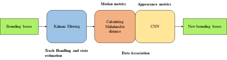
Deep SORT (Simple Online Real-time Tracking with a deep association metric) is an improved version of SORT, is used as a tracker in our tracking by detection approach. It uses conventional vision algorithms to do tracking but by adding deep association metric long term occlusions can be sustained. It is generally assumed the noise to be present in our input data and camera to be uncalibrated. The Deep SORT pipeline is shown in the Figure 3.4.
 |
|---|
| Figure 3.4: Deep SORT Pipeline |
Integration of Detection and Tracking
In tracking-by-detection approach, bounding boxes and tracking IDs are taken from tracking output, but tracking algorithm has generally no influence on class labels. So output class labels have to be fetched from the YOLO output. Number of bounding boxes from YOLO and from tracking will not always be same, as tracking takes care of FPs and FNs . The association between class names and bounding boxes will be a challenge. To mitigate this problem, storing of all class labels will be necessary. For each track, the first frame in which it is being tracked is found and class labels are taken from the stored list. This class label from the first tracked frame will be passed to all consecutive frames until the object is lost.
Results
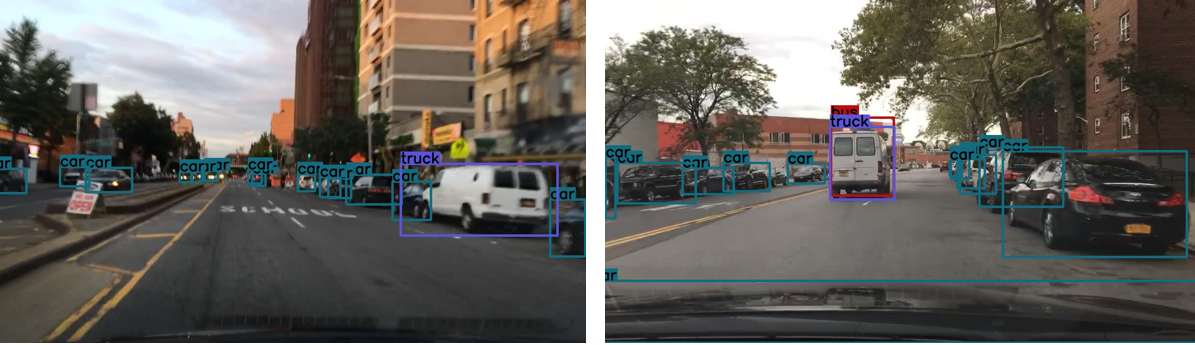
The results of the object detection using YOLO have been shown below.
 |
|---|
| Figure 3.6: Output of YOLO |
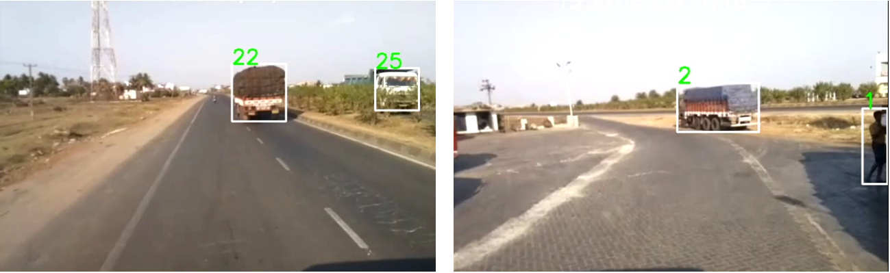
Tracking ID and bounding boxes are generated from tracking. The results of only tracking are shown below.
 |
|---|
| Figure 3.7: Output of Deep SORT |
Results of both tracking and object detection are overlapped and shown below.
 |
|---|
| Figure 3.8: Output of YOLO and Deep SORT |
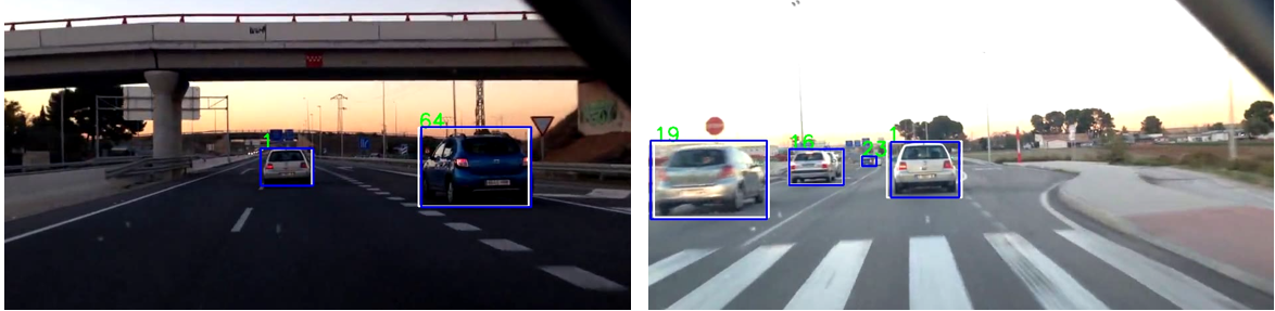
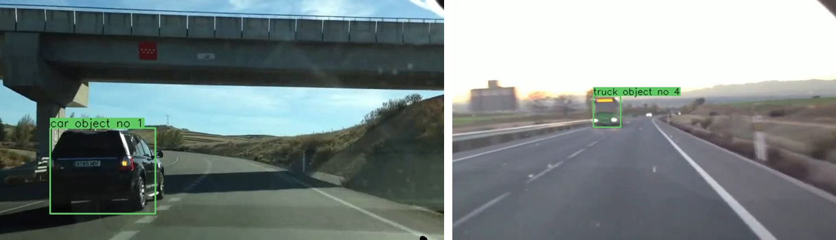
After integration between tracking and detection labels are be shown below. Label contains the class label from YOLO and tracking ID and bounding box from tracker.
 |
|---|
| Figure 3.9: Integration of Object Detection and Tracking Outputs |
Lane Detection
Problem Definition
Deep learning architecture should be able to detect all the lanes and be able to differentiate ego lane from the detected lanes despite partial occlusion. It should be able to predict the precise lane curve.
Need for the Task
The interest to develop lane detection solutions increased with the demand for ADAS and self driving cars. Drivers not only depend on the lanes for safe driving but also for visual cues (e.g., pavement markings) to understand what it is and what is not allowed (e.g., lane change,direction change). The integration part discussed in the later section of the report assumes the lane as an object of reference for detecting ego motion, i.e motion of the camera on board vehicle. Lane detection plays an important part in vehicle lane change activity analysis.
Preamble of the Network Used
To compute spatial relationships, traditionally Markov Random Fields and Conditional Random Fields were used. Message passing, is another spatial relationship computation process wherein each pixel gets information from the pixels around it. It is computationally expensive and harder to be implemented in real time. Generally, these methods are applied to the output of the CNN models. The top hidden layer comprises of rich information which could be a better place for placing the spatial relationship model.The Spatial Convolutional Neural Network (SCNN) offers better run time and spatial relationship model runs over information rich top layer.
Positive Attributes
The positive attributes of SCNN network are as follows :
- The adopted network has the capability to detect the lanes despite partial occlu- sion of lanes.
- SCNN is computationally efficient where message passing is realized in a se- quential propagation scheme rather than each pixel receiving information from the pixels around it.
- It shows good ability to predict fine lane curves and offers good balance between speed (fps) and accuracy.
- It is capable of detecting upto four lanes and differentiates ego lane from the others.
- It gives output in the form of pixel coordinate location of the detected lanes points which is easier for integration.
Network Architecture
SCNN views rows or columns of feature maps as layers and applies convolution, nonlinear activation, and sum operations sequentially, which forms a deep neural network. This makes it possible for the information to be passed between the neurons in the same layer. The word spatial in SCNN, denotes propagating spatial information via specific CNN structure design.
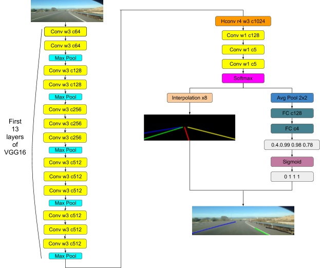
The architecture of the adopted network is shown in the Figure 3.10. The network resizes the input image size to 800×288 by linear interpolation function using OpenCV library and sends it as a 3-D tensor input of size C × H × W , where C, H, and W denote the number of channel, rows and columns respectively. The input tensor is then passed to the first 13 layers of VGG16 and the weights are initialized accordingly from VGG16 model. Followed by atrous convolution of rate 4 which strikes a good balance between efficiency and accuracy. Then fast bilinear interpolation by an additional factor of 8 is done to recover the feature maps at the original resolution. The probability maps from softmax layer is passed over to another small network to predict existence of lane markings. For lanes with more than 0.5 for lane existence value, the network searches every row in the corresponding probability map for the pixel locations with highest response and these locations are then connected by cubic splines. The detected lane pixel coordinates is then overlaid over the actual input image with different color codes for the four lanes. The region between detected blue lane and detected green lane is the ego lane. The metric evaluation of the network is not within the scope of this project.
 |
|---|
| Figure 3.10: SCNN Lane Detection Architecture |
Results
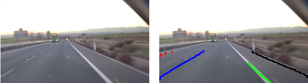
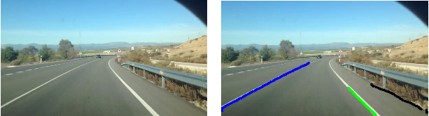
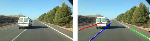
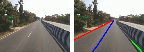
The SCNN algorithm was run on the videosets downloaded from the internet. The ego lane is the path between blue and green detected lanes. The algorithm performed impressively considering the ability to detect lanes despite partial occlusion and different lighting conditions. Figure 3.11, Figure 3.12, Figure 3.13 and Figure 3.14 shows detection results of different lanes subjected to different conditions. There were a few frames with unsatisfactory results Figure 3.15 in which two different lane colors were overlaid on the same lane. When the separation between the dashed lane increases, the algorithm performs unreliably. Also, eccentricity of the lanes has a huge impact in the lane detection.
 |
|---|
| Figure 3.11: SCNN Result for Straight Lanes |
 |
|---|
| Figure 3.12: SCNN Result for Curved Lanes |
 |
|---|
| Figure 3.13: SCNN Result for Partially Occluded Lanes |
 |
|---|
| Figure 3.14: SCNN Result for Lanes Under Shadow |
 |
|---|
| Figure 3.15: Poor Results from SCNN |
OPTICAL FLOW ESTIMATION
Problem Definition
Optical flow is the movement of the brightness patterns across frames caused due to the apparent movement of objects on the real world. The optical flow vector of every pixel in every frame of the acquired video has to be determined by the network.
Need for the Task
Each pixel will have a flow vector will have two components along X and Y directions which are nothing but projections of the actual 3-D flow of the objects on the image. Estimation of this flow is essential as we can extract information about the motion of every object on the scene using this information. The motion of the ego vehicle can also be determined using the static objects (known beforehand) on the scene.
Preamble of the Network Used
Traditionally, optical flow estimation has always been a problem which has been solved using image processing techniques. It was one of the areas of computer vision where deep learning could not make a quick impact. It was largely due to the lack of availability of ground truth. Manual labelling was a laborious and time consuming task as it involved labelling every pixel motion.
Optimizing a complex energy function was the approach used by many of the traditional algorithms but it was computationally expensive. It assumed brightness constancy and spatial smoothness constraints to predict the optical flow. CNNs were initially used as a component in the algorithms to perform tasks such as sparse to dense interpolation, construction of cost volume and sparse matching. The most recent methods used cost volumes, pyramid creation and warping methods but they were not real-time.
Positive Attributes
The positive attributes of PWC-Net are as follows :
- PWC-Net model has computationally light CNN layers, cost volumes and warp- ing compared to energy minimization approaches.
- It constructs only partial cost volume making it more memory and computation efficient.
- It used feature pyramids instead of image pyramids making it invariant to shadows and lighting changes.
- It combines deep learning with domain knowledge to reduce model size as well as improve performance.
Network Architecture
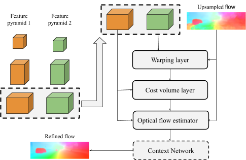
PWC stands for pyramidal processing, warping and cost volume. The method has been designed based on these simple principles. The method can be divided into five major parts - feature pyramid extractor, warping layer, cost volume layer, optical flow estimator and context network.
 |
|---|
| Figure 3.16: PWC-Net Architecture |
Feature pyramid extractor
Two consecutive frames are taken as the two images and n-level pyramids of feature representations are created. The input images are the bottommost images. Layers of convolutional filters are used to downsample the features at each pyramid level by 2. With each level, the number of feature channels keep on doubling starting from 16 for the first level to 196 for the sixth level. Siamese network is used to encode the frames. Leaky ReLU is used as the activation function after every convolutional layer.
Warping layer
At nth level, bilinear interpolation is used to warp the features of the second frame on the first frame using x2 upsampled flow from the n+1 th level. The flow for backpropagation and gradients to CNN features’inputs are computed.
Cost volume layer
Cost volume defines the range of search for corresponding features between the consecutive frames. It stores the costs for matching them appropriately. It is defined as the correlation between the first frame and warped features of second frame. An important thing to note is that the motion at the topmost level of the pyramid amplifies with the decrease in level. A small motion at the top might amplify, to become a significant motion at the actual resolution.
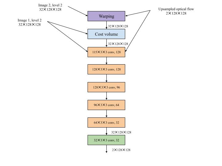
Optical flow estimator
The optical flow estimator is a CNN on its own. Its architecture is shown in Figure 3.17. It is fixed at second level of the pyramid. In this network too, Leaky ReLU is used as the activation function that follows the convolutional layer. The cost volume, first image’s features and upsampled optical flow are the inputs of the network. The number of feature channels keeps on reducing from 128 to 32 with the layers. The final layer does not have any activation function as it provides the output i.e. optical flow at the n th level.
 |
|---|
| Figure 3.17: Optical Flow Estimator Network |
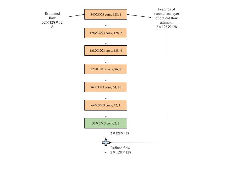
Context network
The context network is used to post process the flow [ Figure 3.18]. This is also applied at the second pyramid level and a leaky ReLU follows each convolutional layer. Its inputs are the estimated optical flow and the penultimate layer’s features from the optical flow estimator network. The dilation constants given at the end handles the separation between the input units in horizontal and vertical directions. The output of the context network is the refined optical flow.
 |
|---|
| Figure 3.18: Context Network |
Results
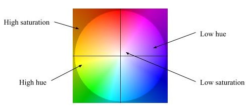
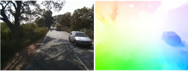
Each pixel will have a 2-D vector which can be converted to polar coordinates for visualization. The visualization is colour coded in such a manner that hue represents direction and saturation represents magnitude of the flow vector as shown in the Figure 3.19. The optical flow output for a sample frame is shown in the Figure 3.20.
 |
|---|
| Figure 3.19: Colour Coding for Optical Flow Visualization |
 |
|---|
| Figure 3.20: Sample Frame and its Optical Flow Output from PWC-Net |
INTEGRATION AND INFERENCE
Object detection and tracking, lane detection and optical flow estimation cannot provide meaningful data on their own separately. Their outputs have to be made use of to extract meaningful data about vehicle activity and acquire the final labels. This integration of outputs from all the three aforementioned networks majorly involves the use of image processing techniques and pixel level processing.
Metrics involves quantifying the various numerical parameters such as distance, speed, etc. but semantics involves just qualitative labelling. Semantics can just provide information about whether a change is happening or not. It cannot provide how fast or how slow the change is happening as it would all be relative. The work carried out in this project involves extracting semantic labels for vehicle activity as metric labels are not possible to acquire using the data from just a single camera. There are various techniques to estimate the depth, get metrics about distance of objects on the scene, etc. but they are not reliable and robust to be performed using just a single camera. Moreover, the recent trend in autonomous driving is to do more with just a single camera. Autonomous vehicle makers such as Tesla are aspiring towards it. Hence, the labels given for every vehicle would be semantic and the details are discussed in Figure 4.1.
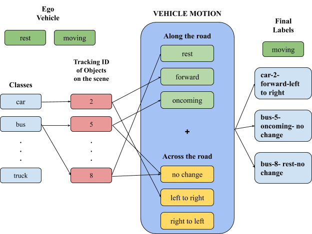
Figure 4.1 shows how the final label for each vehicle is obtained. The final label consists of two parts.
- The first label describes the motion of the ego vehicle itself, if it is at rest or moving and is displayed at the bottom of each frame.
- The second label is for each and every vehicle and follows the following format: class name - tracking ID - along the road - across the road.
The class name of the object is the first part of the label which is obtained from YOLOv3. The tracking ID for the corresponding object is obtained from DeepSORT and appended to the class name. The labels to describe vehicle motion along the road and across the road are appended at the end.
 |
|---|
| Figure 4.1: Final Output Labels |
VEHICLE MOTION ALONG THE ROAD
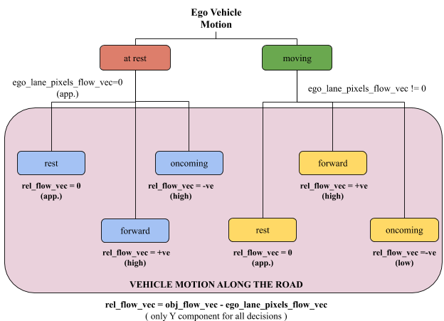
The third part of the final label for each vehicle is the motion of the vehicle along the road. This is an important part where the results from optical flow matters a lot. The decision tree for prediction of vehicle motion along the road is shown in Figure 4.2.
 |
|---|
| Figure 4.2: Decision Tree for Prediction of Vehicle Motion Along the Road |
Reference Frame
First of all, to define any motion, a reference frame has to be set. In this case, the lane markings on the road are considered as the reference for all motion as they are stationary. The ego vehicle motion and motion of the vehicles on the scene are predicted with reference to these lane markings.
Decision Tree Level 0
If the ego vehicle is at rest, the ego lane markings detected by the lane marking detection network will also be stationary. Hence, their flow vector will have zero magnitude. If the vehicle is at motion, the lane markings will have a considerable amount of flow in the negative Y direction.
Decision Tree Level 1
Once the ego vehicle motion is decided, there are three possibilities of motion for the vehicle on scene in each case - rest, forward and oncoming. For this level, a relative optical flow vector is obtained where the Y component of the flow vector of the ego lane pixels are subtracted from the Y component of the flow vector of the object.
Note that in both the levels of the decision tree, the flow vector average of only the ego lane markings are considered as the other lanes are too eccentric and reduce the average magnitude of the lane flow vector. The relative flow vector obtained is used to decide the motion of the vehicle. It can be almost equal to zero, have a positive value (high or low) or a negative value (high or low) depending on the cases presented in Figure 4.2.
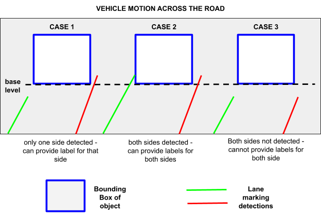
VEHICLE MOTION ACROSS THE ROAD
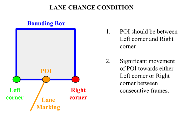
The fourth and the final label for each vehicle describes its motion across the lane. Due to perspective projection, even if a vehicle moves far away from the ego vehicle without changing lane, still there would be a component of optical flow along the X direction. Hence, using optical flow for this case proves to be ambiguous. Hence, a different approach is taken here given by the following Figure 4.4.
 |
|---|
| Figure 4.4: Lane Change Condition |
Two conditions have to be satisfied to provide the lane change label. The point of intersection of the lane marking and the bounding box of the object should be between the left and right bottommost corners of the bounding box. This condition proves that the vehicle is not travelling in one specific lane. The second condition is that the point of intersection should move significantly towards either the left or the right corner between successive frames and the labels like ( left to right or right to left ) can be given according to that. In case there is no significant movement, then no change will be alloted as the label. Various cases for lane changing prediction are shown in the Figure 4.3.
 |
|---|
| Figure 4.3: Cases for Lane Changing Prediction |
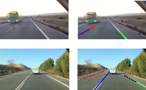
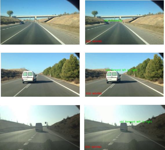
In any case, the tracking ID will always be available on the final label. The class name might be missing in a few frames but it is a rare occurrence as YOLO detects almost all object accurately across all frames. The labels for vehicle motion along and across the road will also be present for all the frames as it covers all the cases.The final output with labels for few sample frames are shown in Figure 4.5.
 |
|---|
| Figure 4.5: Final Results with Labels |
INFERENCING
Inferencing for final integration was carried out on both embedded platform and PC for video sets obtained from internet sources. The processing was done frame by frame. Since PC offers external GPU support, inferencing was done much faster done on PC.
Inferencing on Embedded Platform
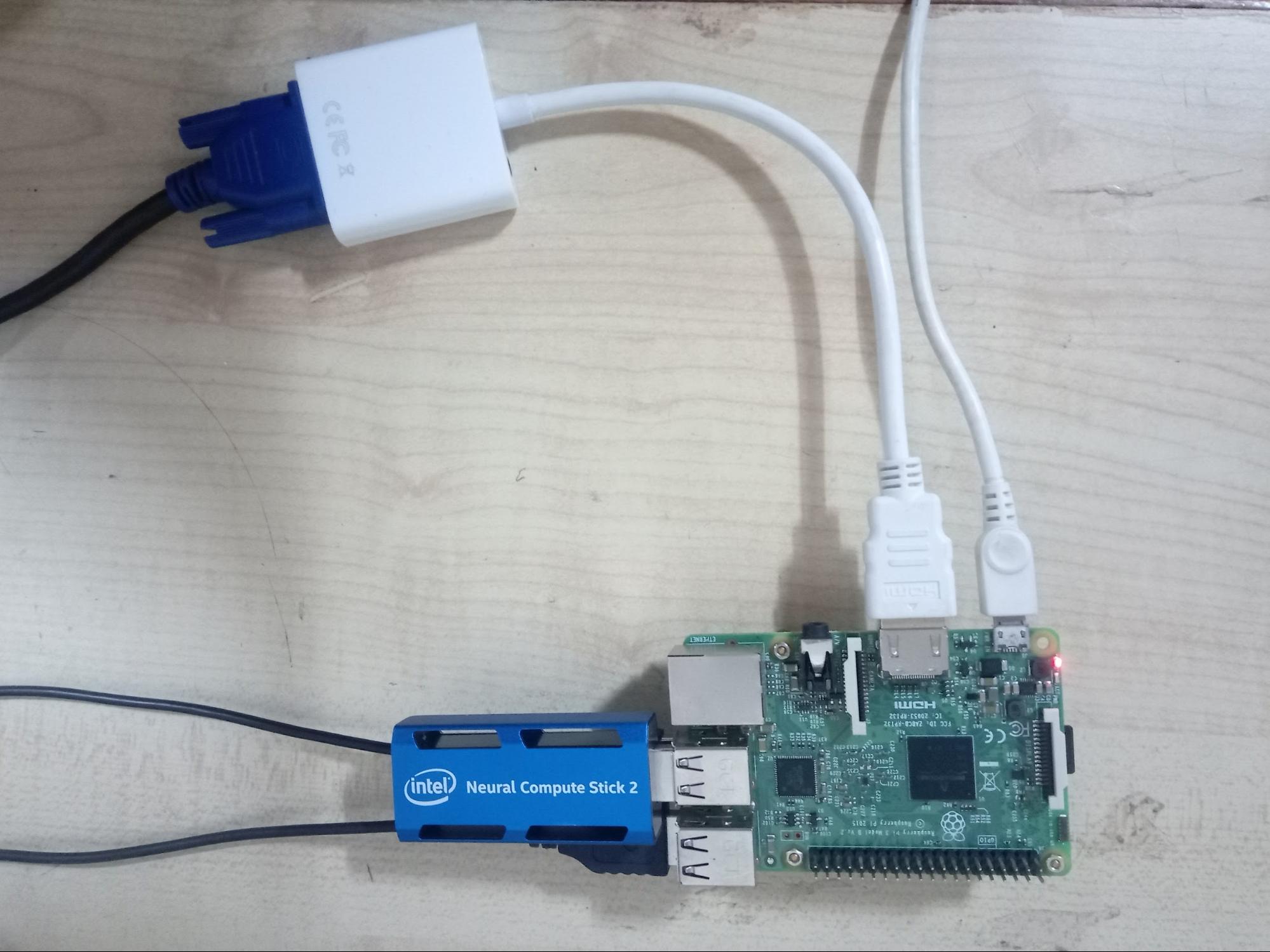
Raspberry Pi model 3B [Table 4.1] was chosen as the primary processor which is assisted by the Intel Neural Compute Stick-2 to run deep neural networks [Figure 4.6]. Intel NCS-2 which is powered by Intel’s VPU(Vision Processing Unit) - the Intel Movidius Myriad X, which includes an on-chip neural network accelerator called the Neural Compute Engine. It has 16 programmable SHAVE (Streaming Hybrid Architecture Vector Engine) cores which accelerates the deep learning network performance. Deployment of the models on NCS required installation of the Intel Openvino toolkit and conversion of checkpoint files to XML and binary files.
Table 4.1: Embedded Platform Specifications
| Device Model | Raspberry pi 3B |
|---|---|
| Central Processing Unit (CPU) | 4 X ARM Cortex-A53, 1.2GHz |
| GPU | Broadcom VideoCore IV |
| RAM | 1GB LPDDR2 (900 MHz) |
| Storage | 32GB micro SD card class 10 |
| Power supply | 6V 2-3A |
| Operating System | Raspbian Stretch |
 |
|---|
| Figure 4.6: Embedded Hardware with Intel NCS-2 |
NCS is a relatively new device specifically designed for the inferencing of deep neural networks. Some of the layers of Neural networks such as argmax, etc. are not supported by it due to reasons not known yet. The available online community support is also less. It has USB form factor and can be plugged directly into the Raspberry Pi.
It ran at 2 fps for YOLOv3. Due to the lack of support of some layers, PWCNet and SCNN could not be deployed on NCS. However, future work could be done to modify these layers to suit the NCS.
Inferencing on PC
The integration script was run on PC which reads the video and processes it frame by frame. Each network is called for every frame and the output data is obtained from them. The CPU and GPU specifications for inference are the same as the one mentioned in Chapter 3 (Table 3.1, Table 3.2). The speed of inference was 5 fps.
Table 3.1: CPU Specifications
| Type | Specification |
|---|---|
| Motherboard | ASUS A68HM-K |
| Processor | AMD A6-7400K Radeon R5, 6 Compute Cores 2C+4G |
| Frequency | 3500 MHz |
| Datapath width | 64-bit |
| System memory | DIMM DDR3 16GB (2x8GB), 600 MHz |
| Storage | Kingston A400 120GB SATA 3 2.5 Solid State Drive |
Table 3.2: GPU Specifications
| Type | Specification |
|---|---|
| Number of CUDA cores | 4352 |
| Number of tensor cores | 544 |
| Single precision performance | 13.4 TFLOPs |
| Memory | 11GB GDDR6 |
| Memory Speed | 14 Gbps |
| Base Clock | 1350 MHz |
| Boost Clock | 1545 MHz |
Conclusion and Future Scope
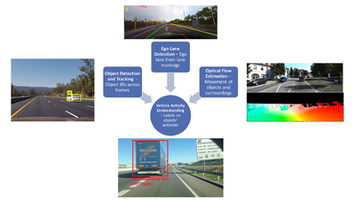
The objective of the project was to interpret the semantic activity of vehicles on the scene. Initially drivable area detection was chosen as the task to understand the road environment but later ego lane detection proved out to be more efficient and computationally less expensive. The three algorithms based on deep neural networks were chosen among the different research articles on the basis of run time, model complexity and accuracy. The outputs of the three networks are integrated to predict the semantic vehicle activity.
The inferred labels were accurate for most test cases but some of the videos had very noisy output, i.e. labels varied in a drastic manner. The result of the integration was heavily dependent on the accuracy of three networks. In some of the frames, YOLO was not able to detect the object but Deep SORT was able to predict the bounding box. As a result, the classes were not identified in those frames. The output of the ego lane detection was affected by eccentric lane markings. The lane detection algorithm struggles to detect when the separation between the dashed lane markings increases.
The embedded implementation was carried on raspberry pi supported by Intel NCS-2 to boost the inference process.The processing frame rate was lower than expected which can be attributed to the complexity of the neural networks and limitations of the processor. One of the major setbacks was that some of the layers of the neural networks were not supported by the Intel NCS-2 and hence some models could not be run on the NCS-2.
This project work can further be enhanced in the following ways :
- Smoothening the output of the integration to make it less noisy
- Training the networks to get best accuracy, preferably with Indian road data.
- Making the DNN pipeline end-to-end, instead of manual integration.
- Making it work in real-time on an embedded board for true real time performance.
Madhu Korada
MRSD Student
My research interests include Computer Vision, EdgeAI algorithms, ADAS and robotics.